Decision Trees, A Bird’s Eye View And An Implementation

What is achieved in this article?

• Understanding the definition of Decision Trees
• Implementation
  • Loading the data
  • Visualizing the data using a correlation matrix and a pair plot
  • Building a Decision Tree Classifier
  • Determining the accuracy of the model using a confusion matrix
  • Visualizing the Decision tree as a flow chart

What are Decision Trees?

A decision tree is a flowchart-like structure in which each internal node represents a “test” on an attribute (e.g. whether a coin flip comes up heads or tails), each branch represents the outcome of the test, and each leaf node represents a class label (decision taken after computing all attributes).

(Source: Wikipedia)

In simpler terms, a decision tree checks if an attribute or a set of attributes satisfy a condition and based on the result of he check, the subsequent checks are performed. The tree splits the data into different parts based these checks.

Implementation

Importing the necessary libraries

import pandas as pd
import numpy as np
from sklearn.preprocessing import StandardScaler
import tflearn.data_utils as du
from sklearn.tree import DecisionTreeClassifier
from sklearn.model_selection import train_test_split
import seaborn as sns
from sklearn.metrics import confusion_matrix

from sklearn.externals.six import StringIO  
from IPython.display import Image  
from sklearn.tree import export_graphviz
import pydotplus

Reading the dataset

data = pd.read_csv('../input/column_3C_weka.csv')

The dataset used here is the Biomechanical features of orthopedic patients

What is correlation?

Correlation is a statistical term which represents the extent of linear relationship between two features.

For example, two variable which are linearly dependent (say, x and y which depend on each other as x = 2y) will have a higher correlation than two variables which are non-linearly dependent (say, u and v which depend on each other as u = sqr(v)).

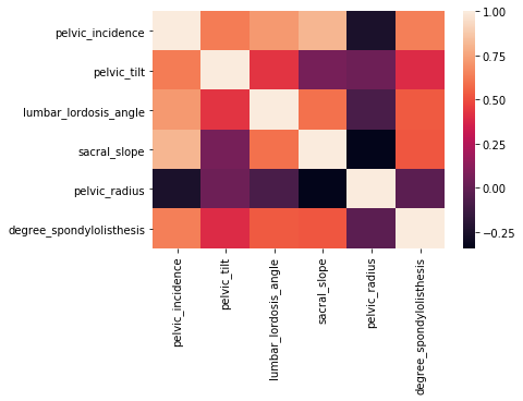
Visualizing the correlation

# Calculating the correlation matrix
corr = data.corr()
# Generating a heatmap
sns.heatmap(corr,xticklabels=corr.columns, yticklabels=corr.columns)

sns.pairplot(data)

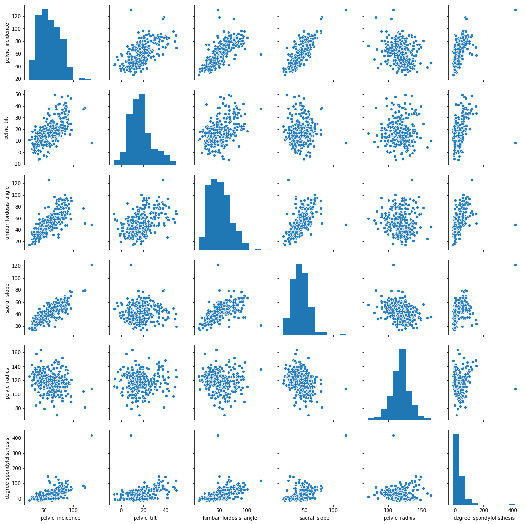
In the above two plots you can clearly see that the pairs of independent variables with a higher correlation have a more linear scatter plot than the independent variables having a relatively lesser correlation.

Splitting the dataset into independent (x) and dependent (y) variables

x = data.iloc[:,:6].values
y = data.iloc[:,6].values

Splitting the dataset into train and test data

x_train , x_test, y_train, y_test = train_test_split(x, y, test_size = 0.25, random_state = 0)

Scaling the independent variables

This question on stackoverflow has responses which gives a brief explanation on why scaling is necessary and how it can affect the model.

sc = StandardScaler()
x_train = sc.fit_transform(x_train)
x_test = sc.transform(x_test)

Building the Decision tree

The criterion here is entropy. The criterion parameter determines the function to measure the quality of a split. When the entropy is used as a criterion, each split tries to reduce the randomness in that part of the data.

There are lot of parameters in the Decision Tree Class that you can tweak to improve your results. There we take a peak into the max_depth parameter.

The max_dept the determines how deep a tree can go. The affect of this parameter on the model will be discusses later in this article

classifier = DecisionTreeClassifier(criterion = 'entropy', max_depth = 4)
classifier.fit(x_train, y_train)

Evaluating the model

Making the prediction on the test data

y_pred = classifier.predict(x_test)

What is a confusion matrix?

A confusion matrix is a technique for summarizing the performance of a classification algorithm. Classification accuracy alone can be misleading if you have an unequal number of observations in each class or if you have more than two classes in your dataset. Calculating a confusion matrix can give you a better idea of what your classification model is getting right and what types of errors it is making.

Source

cm = confusion_matrix(y_test, y_pred)
accuracy = sum(cm[i][i] for i in range(3)) / y_test.shape[0]
print("accuracy = " + str(accuracy))

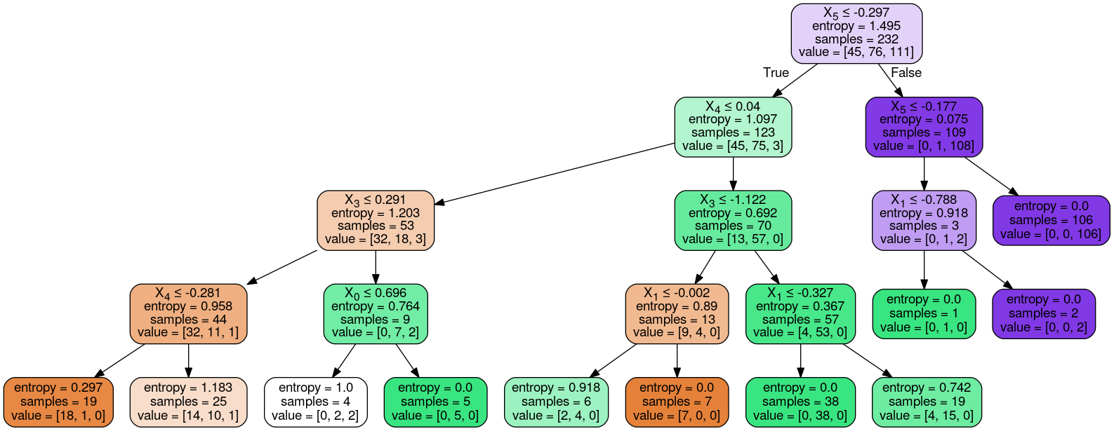
Visualizing the Decision Tree

dot_data = StringIO()
export_graphviz(classifier, out_file=dot_data,  
                filled=True, rounded=True,
                special_characters=True)
graph = pydotplus.graph_from_dot_data(dot_data.getvalue())  
Image(graph.create_png())

Building a model without the max_depth parameter

classifier2 = DecisionTreeClassifier(criterion = 'entropy')
classifier2.fit(x_train, y_train)
y_pred2 = classifier2.predict(x_test)
cm2 = confusion_matrix(y_test, y_pred2)
accuracy2 = sum(cm2[i][i] for i in range(3)) / y_test.shape[0]
print("accuracy = " + str(accuracy2))

Visualizing the decision tree without the max_depth parameter

dot_data = StringIO()
export_graphviz(classifier2, out_file=dot_data, filled=True, rounded=True, special_characters=True)
graph = pydotplus.graph_from_dot_data(dot_data.getvalue())  
Image(graph.create_png())

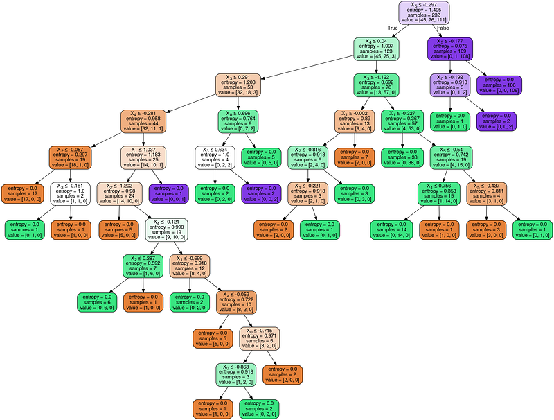
Now, consider the leaf nodes (terminal nodes) of the tree with and without the max_depth parameter. You will notice that the entropy all the terminal nodes are zero in the tree without the max_depth parameter and non zero in three with that parameter. This is because when the parameter is not mentioned, the split recursively takes place till the terminal node has an entropy of zero.

To know more about the different parameters of the sklearn.tree.DecisionTreeClassifier, click here

To get this article as a iPython Notebook, click here and fork it.