Autobound Phase 2 Complete

The second evaluation of Google Summer of Code is complete and the results came out a week back. This article explains what I did during the second phase of GSoC building AutoBound.
The main two main tasks I focused on during the second phase of GSoC were:

1. Data Collection
   
2. The plugin-server pipeline

Data Collection

The plugin and server ends for data collection were completed during the first phase of GSoC. So, here I will explain the workflow for collecting data I used.
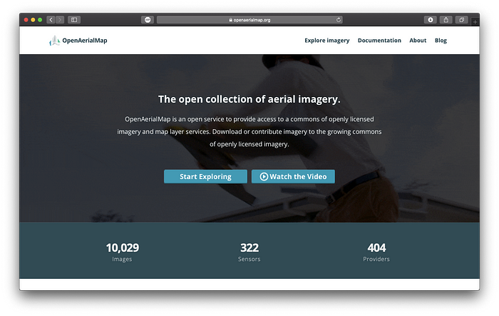
To train the model, I needed high res aerial images and good data. I got them from OpenAerialMap and OpenStreetMap respectively. I filtered the latest, high res aerial imagery available in OpenAerialMap. But this was not enough. The area I download must have buildings and good data in OSM. I found that European countries generally satisfied both these conditions. So, I used JOSM’s remote control to open the imagery and corresponding data in JOSM. Sometimes JOSM will throw an error saying the download area is too large. in that case, open the area in iD and zoom to the area with the imagery. Now, use remote control to open that area in JOSM. Add the imagery to JOSM from OpenAerialMap.

Now use the Collect Data — AutoBound option from the Tools menu to start collecting the data.
Sometimes due to poor internet connectivity, some images may not be downloaded properly or, the data or the area might not match with the imagery. I had to manually delete such data. To make this easier, I built another small tool (Not a great one but gets the job done) — ManualImageSelector. This will show you the original image and segmented image side by side so you can compare and decide if you want to keep the image or not.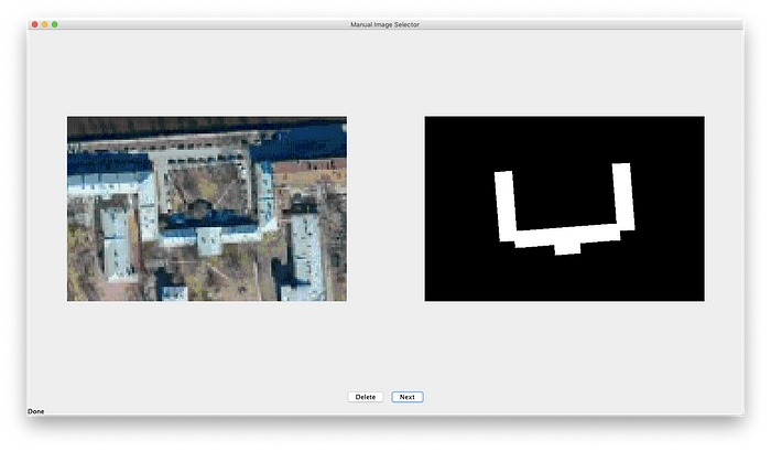

Plugin Server

This is an important part of AutoBound. During deployment, the image extracted by JOSM must be processed, sent to the server, processed again there and the results must be sent back to the plugin. Building this entire pipeline was the second and more important task during the second phase of GSoC.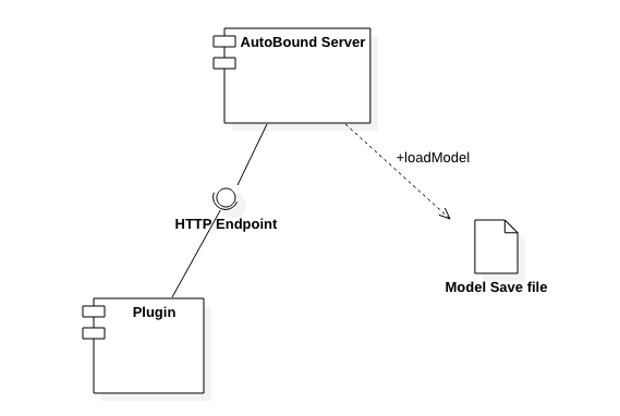

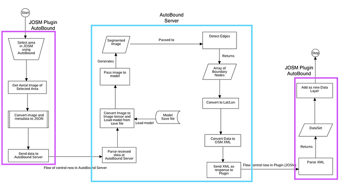
The code to send data to the server and process the received data was done during the first phase of GSoC. Now the server side was the one that needed building. The image was sent to the server in a base64 encoded format. This image is decoded. Next the model is loaded from a save file. The model used by the server is an untrained resnet 101 (This will be replaced with a trained s and possibly simpler model during the third phase). Fast.ai’s vision.data modules are used to load and preprocess the image. The image is then passed to the model to generate the segmented image (which right now is just random). This image is then processed to get the edges. These edges are then converted to lat/lon coordinates. These coordinates are converted to JOSM-XML. This XML is then sent back to the plugin where it is parsed, added as a new DataLayer and displayed on the MapView.
This concludes the work during the second phase of Google Summer of Code.
In the next phase, I am collecting more data, building and training a model for the server. Expect a post on my progress and updates soon.